The first classifier, and — despite the name — a classification model rather than a regression one. It keeps linear regression's weighted sum and adds two things: a function that squashes that sum into \([0,1]\), and a loss built for probabilities instead of distances.
It remains the default first model for binary classification on tabular data: fast, calibrated out of the box (8.7), and the only classifier in this material whose coefficients can be read directly.
import numpy as np
import pandas as pd
import matplotlib.pyplot as plt
import seaborn as sns

from sklearn.linear_model import LogisticRegression
from sklearn.pipeline import make_pipeline
from sklearn.preprocessing import StandardScaler
from sklearn.model_selection import StratifiedKFold, cross_val_score, train_test_split
from sklearn.metrics import accuracy_score, log_loss, roc_auc_score

RANDOM_STATE = 42
rng = np.random.default_rng(RANDOM_STATE)

np.set_printoptions(precision=4, suppress=True)
pd.set_option("display.width", 115)
sns.set_theme(style="whitegrid")

cv = StratifiedKFold(5, shuffle=True, random_state=RANDOM_STATE)
print("ready")
ready
13.1 From Regression to Classification
The obvious idea is to fit a linear regression to a 0/1 target and threshold its output at 0.5. It fails in two specific ways, and both are worth seeing before the fix.
from sklearn.linear_model import LinearRegression

# Hours studied vs pass/fail.
hours = np.array([0.5, 1.0, 1.5, 2.0, 2.5, 3.0, 3.5, 4.0, 4.5, 5.0, 5.5, 6.0]).reshape(-1, 1)
passed = np.array([0, 0, 0, 0, 0, 1, 0, 1, 1, 1, 1, 1])

linear = LinearRegression().fit(hours, passed)

probe = np.array([[-1.0], [0.0], [3.0], [9.0], [12.0]])
for xv, pred in zip(probe.ravel(), linear.predict(probe)):
    flag = "   <- not a probability" if pred < 0 or pred > 1 else ""
    print(f"hours {xv:>5.1f}  ->  {pred:>7.3f}{flag}")
hours  -1.0  ->   -0.510   <- not a probability
hours   0.0  ->   -0.273   <- not a probability
hours   3.0  ->    0.441
hours   9.0  ->    1.867   <- not a probability
hours  12.0  ->    2.580   <- not a probability
Failure 1 — the output is unbounded. A linear function extends forever in both directions, so it predicts negative "probabilities" for small inputs and values above 1 for large ones. There is no interpretation of \(-0.28\) as a probability.
Failure 2 — outliers rotate the decision boundary. Squared loss penalizes a confidently-correct point that sits far from the line, so adding a student who studied for 25 hours and passed drags the boundary even though it adds no new information about where the boundary should be.
hours_ext = np.vstack([hours, [[25.0]]])
passed_ext = np.r_[passed, 1]

linear_ext = LinearRegression().fit(hours_ext, passed_ext)

def boundary(model):
    """Where does the fitted line cross 0.5?"""
    return (0.5 - model.intercept_) / model.coef_[0]

print(f"linear boundary, without the distant point: {boundary(linear):.2f} hours")
print(f"linear boundary, with it                  : {boundary(linear_ext):.2f} hours")

logit = LogisticRegression().fit(hours, passed)
logit_ext = LogisticRegression().fit(hours_ext, passed_ext)
print(f"\nlogistic boundary, without : "
      f"{-logit.intercept_[0] / logit.coef_[0][0]:.2f} hours")
print(f"logistic boundary, with    : "
      f"{-logit_ext.intercept_[0] / logit_ext.coef_[0][0]:.2f} hours")
linear boundary, without the distant point: 3.25 hours
linear boundary, with it                  : 3.94 hours

logistic boundary, without : 3.25 hours
logistic boundary, with    : 3.25 hours
grid = np.linspace(-1, 12, 300).reshape(-1, 1)

fig, ax = plt.subplots(figsize=(6.5, 3.8))
ax.scatter(hours, passed, s=40, zorder=3, label="data")
ax.plot(grid, linear.predict(grid), label="linear regression")
ax.plot(grid, logit.predict_proba(grid)[:, 1], label="logistic regression")
ax.axhline(0, color="gray", lw=0.7); ax.axhline(1, color="gray", lw=0.7)
ax.axhline(0.5, color="tab:red", ls=":", lw=1, label="threshold 0.5")
ax.set_xlabel("hours studied"); ax.set_ylabel("P(pass)")
ax.set_title("Linear regression leaves [0, 1]; the logistic curve cannot")
ax.legend(fontsize=8)
fig.tight_layout()
plt.show()
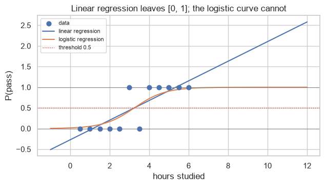
The fix for both failures is the same: pass the linear score through a function that is bounded, and replace squared loss with one built for probabilities.
13.2 The Sigmoid, Odds and Log-Odds
The logistic (sigmoid) function maps any real number into \((0, 1)\):
\[\sigma(z) = \frac{1}{1 + e^{-z}}\]
| \(z\) | \(\sigma(z)\) |
|---|---|
| \(-\infty\) | 0 |
| \(-2\) | 0.12 |
| 0 | 0.5 |
| \(+2\) | 0.88 |
| \(+\infty\) | 1 |
The model is then linear regression's score fed through it:
\[\hat{p} = P(y = 1 \mid \mathbf{x}) = \sigma(\mathbf{w}\cdot\mathbf{x} + b)\]
def sigmoid(z):
    return 1 / (1 + np.exp(-z))


for z in (-6, -2, -1, 0, 1, 2, 6):
    print(f"sigmoid({z:>3}) = {sigmoid(z):.4f}")

print("\nbounded:", sigmoid(-1000), "to", sigmoid(1000))
print("symmetric about 0:", np.isclose(sigmoid(2) + sigmoid(-2), 1.0))
sigmoid( -6) = 0.0025
sigmoid( -2) = 0.1192
sigmoid( -1) = 0.2689
sigmoid(  0) = 0.5000
sigmoid(  1) = 0.7311
sigmoid(  2) = 0.8808
sigmoid(  6) = 0.9975

bounded: 0.0 to 1.0
symmetric about 0: True
z = np.linspace(-8, 8, 400)
fig, axes = plt.subplots(1, 2, figsize=(10, 3.2))

axes[0].plot(z, sigmoid(z))
axes[0].axhline(0.5, color="tab:red", ls=":"); axes[0].axvline(0, color="gray", lw=0.7)
axes[0].set_xlabel("z = w.x + b"); axes[0].set_ylabel("sigma(z)")
axes[0].set_title("the sigmoid", fontsize=10)

axes[1].plot(z, sigmoid(z) * (1 - sigmoid(z)))
axes[1].set_xlabel("z"); axes[1].set_ylabel("sigma'(z)")
axes[1].set_title("its derivative: steepest at z = 0, flat in the tails", fontsize=10)

fig.tight_layout()
plt.show()
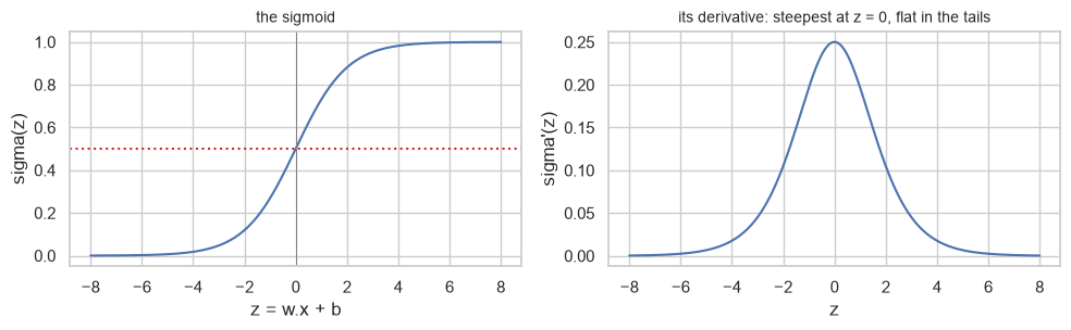
The derivative has a convenient closed form that 13.4 uses directly:
\[\sigma'(z) = \sigma(z)\,(1 - \sigma(z))\]
h = 1e-6
numerical = (sigmoid(z + h) - sigmoid(z - h)) / (2 * h)
analytic = sigmoid(z) * (1 - sigmoid(z))
print("analytic derivative matches numerical:", np.allclose(analytic, numerical))
analytic derivative matches numerical: True
13.2.1 Odds and log-odds
The sigmoid has an inverse, and the inverse is what makes the coefficients interpretable.
Odds are the ratio of the probability of an event to its complement:
\[\text{odds} = \frac{p}{1-p}\]
Taking the logarithm gives the log-odds, or logit — and rearranging the model shows that the linear score is the log-odds:
\[\log\!\frac{\hat{p}}{1-\hat{p}} = \mathbf{w}\cdot\mathbf{x} + b = z\]
| Probability | Odds | Log-odds |
|---|---|---|
| 0.10 | 1 : 9 = 0.11 | −2.20 |
| 0.25 | 1 : 3 = 0.33 | −1.10 |
| 0.50 | 1 : 1 = 1.00 | 0 |
| 0.75 | 3 : 1 = 3.00 | +1.10 |
| 0.90 | 9 : 1 = 9.00 | +2.20 |
This is the sentence that makes logistic regression interpretable: the model is linear in the log-odds. A one-unit increase in \(x_j\) adds \(w_j\) to the log-odds, which multiplies the odds by \(e^{w_j}\) (13.8).
def logit_fn(p):
    return np.log(p / (1 - p))


for p in (0.1, 0.25, 0.5, 0.75, 0.9):
    print(f"p = {p:.2f}   odds = {p / (1 - p):>6.3f}   log-odds = {logit_fn(p):>7.4f}")

print("\nlogit and sigmoid are inverses:", np.allclose(sigmoid(logit_fn(0.37)), 0.37))
p = 0.10   odds =  0.111   log-odds = -2.1972
p = 0.25   odds =  0.333   log-odds = -1.0986
p = 0.50   odds =  1.000   log-odds =  0.0000
p = 0.75   odds =  3.000   log-odds =  1.0986
p = 0.90   odds =  9.000   log-odds =  2.1972

logit and sigmoid are inverses: True
13.3 Maximum Likelihood and Cross-Entropy
11.2 chose squared loss because it is the maximum-likelihood estimate under Gaussian noise. The same principle, applied to a binary target, gives a different loss.
Each observation is a Bernoulli trial (2.7.2) with success probability \(\hat{p}^{(i)}\), so the likelihood of the whole dataset is
\[L(\mathbf{w}) = \prod_{i=1}^{n} \left(\hat{p}^{(i)}\right)^{y^{(i)}} \left(1 - \hat{p}^{(i)}\right)^{1 - y^{(i)}}\]
That exponent trick is just a switch: when \(y^{(i)} = 1\) the term is \(\hat{p}^{(i)}\), and when \(y^{(i)} = 0\) it is \(1 - \hat{p}^{(i)}\).
Multiplying thousands of probabilities underflows to exactly zero (2.9.3), so take logs — which also turns the product into a sum. Negating to get something to minimize gives the binary cross-entropy, or log loss:
\[\boxed{\;J(\mathbf{w}) = -\frac{1}{n}\sum_{i=1}^{n}\left[y^{(i)}\log \hat{p}^{(i)} + \left(1 - y^{(i)}\right)\log\left(1 - \hat{p}^{(i)}\right)\right]\;}\]
This is 8.5.3's metric and 10.2.2's surrogate loss — the same function, arrived at from three directions.
def binary_cross_entropy(y_true, p_pred, eps=1e-15):
    p = np.clip(p_pred, eps, 1 - eps)             # clip: log(0) is -inf
    return -np.mean(y_true * np.log(p) + (1 - y_true) * np.log(1 - p))


y_demo = np.array([1, 1, 0, 0])
for label, preds in (("confident and right", [0.95, 0.95, 0.05, 0.05]),
                     ("hesitant", [0.6, 0.6, 0.4, 0.4]),
                     ("confident and WRONG", [0.05, 0.05, 0.95, 0.95])):
    print(f"{label:<22} log loss {binary_cross_entropy(y_demo, np.array(preds)):.4f}")
confident and right    log loss 0.0513
hesitant               log loss 0.5108
confident and WRONG    log loss 2.9957
Confident mistakes are punished far harder than hesitant ones — the asymmetry 8.5.3 showed, and the reason logistic regression produces well-calibrated probabilities rather than merely correct labels.
Check against scikit-learn:
p_demo = np.array([0.9, 0.7, 0.2, 0.1])
print(f"from scratch : {binary_cross_entropy(y_demo, p_demo):.10f}")
print(f"scikit-learn : {log_loss(y_demo, p_demo):.10f}")
print("agree:", np.isclose(binary_cross_entropy(y_demo, p_demo), log_loss(y_demo, p_demo)))
from scratch : 0.1976348816
scikit-learn : 0.1976348816
agree: True
13.3.1 The gradient
Substituting \(\hat{p} = \sigma(X\mathbf{w})\) into the cross-entropy and differentiating gives a result that is almost suspiciously tidy:
\[\nabla J = \frac{1}{n} X^\top \left(\sigma(X\mathbf{w}) - y\right)\]
This is the same form as linear regression's gradient (11.2.2), with \(\sigma(X\mathbf{w})\) in place of \(X\mathbf{w}\) and without the factor of 2. The sigmoid's derivative \(\sigma(1-\sigma)\) cancels exactly against a matching term from the log — which is not a coincidence but a property of the exponential family.
2.6.2's habit applies: verify it numerically before trusting it.
def add_intercept(X):
    return np.column_stack([np.ones(len(X)), X])


def logistic_loss(X, y, w):
    return binary_cross_entropy(y, sigmoid(X @ w))


def logistic_gradient(X, y, w):
    return X.T @ (sigmoid(X @ w) - y) / len(y)


X_check = rng.normal(size=(60, 3))
y_check = (rng.random(60) < sigmoid(X_check @ np.array([1.0, -2.0, 0.5]))).astype(int)
Xd_check = add_intercept(X_check)
w_probe = np.array([0.3, -0.4, 0.8, 0.1])

h = 1e-6
numerical = np.array([
    (logistic_loss(Xd_check, y_check, w_probe + h * np.eye(4)[j])
     - logistic_loss(Xd_check, y_check, w_probe - h * np.eye(4)[j])) / (2 * h)
    for j in range(4)
])

print("analytic :", logistic_gradient(Xd_check, y_check, w_probe))
print("numerical:", numerical)
print("agree:", np.allclose(logistic_gradient(Xd_check, y_check, w_probe), numerical))
analytic : [-0.0704 -0.1979  0.372   0.0871]
numerical: [-0.0704 -0.1979  0.372   0.0871]
agree: True
There is no closed form. Setting \(\nabla J = 0\) gives a system with \(\sigma\) wrapped around the
parameters, which cannot be solved algebraically as 11.2.2's could. Logistic regression is therefore
always fitted iteratively (Chapter 10) — which is why it has max_iter, a solver choice, and a
ConvergenceWarning, and linear regression has none of those.
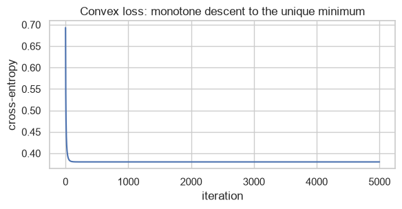
The loss is still convex (10.3), so the iterative solution is unique regardless of initialization.
13.4 Logistic Regression from Scratch
Gradient descent (10.4) with the gradient just verified. That is the entire algorithm.
def fit_logistic(X, y, lr=0.5, n_iter=5000):
    """Batch gradient descent on the cross-entropy. X has NO intercept column."""
    Xd = add_intercept(X)
    w = np.zeros(Xd.shape[1])
    history = np.empty(n_iter)
    for i in range(n_iter):
        history[i] = logistic_loss(Xd, y, w)
        w -= lr * logistic_gradient(Xd, y, w)
    return w, history


def predict_proba_scratch(X, w):
    return sigmoid(add_intercept(X) @ w)


# A clean synthetic problem with known coefficients.
n = 800
X_lr = rng.normal(size=(n, 3))
W_TRUE = np.array([-0.5, 2.0, -1.5, 1.0])           # intercept first
y_lr = (rng.random(n) < sigmoid(add_intercept(X_lr) @ W_TRUE)).astype(int)

w_scratch, history = fit_logistic(X_lr, y_lr)

print("true        :", W_TRUE)
print("from scratch:", w_scratch)
print(f"\nfinal log loss: {history[-1]:.6f}")
print(f"class balance : {y_lr.mean():.3f}")
true        : [-0.5  2.  -1.5  1. ]
from scratch: [-0.3825  1.8692 -1.757   0.8649]

final log loss: 0.379891
class balance : 0.443
Step 4 of the contract. scikit-learn regularizes by default (C=1.0), so the comparison needs
penalty=None to fit the same objective.
sk = LogisticRegression(C=np.inf, max_iter=10_000).fit(X_lr, y_lr)
sk_params = np.r_[sk.intercept_, sk.coef_[0]]

print("from scratch :", w_scratch)
print("scikit-learn :", sk_params)
print(f"\nmax absolute difference: {np.abs(w_scratch - sk_params).max():.2e}")
print("agree to 3 decimals:", np.allclose(w_scratch, sk_params, atol=1e-3))
from scratch : [-0.3825  1.8692 -1.757   0.8649]
scikit-learn : [-0.3825  1.8691 -1.7564  0.8648]

max absolute difference: 6.88e-04
agree to 3 decimals: True
p_scratch = predict_proba_scratch(X_lr, w_scratch)
p_sk = sk.predict_proba(X_lr)[:, 1]

print(f"max difference in predicted probabilities: {np.abs(p_scratch - p_sk).max():.2e}")
print(f"log loss, from scratch : {log_loss(y_lr, p_scratch):.8f}")
print(f"log loss, scikit-learn : {log_loss(y_lr, p_sk):.8f}")
print(f"accuracy agreement     : {np.mean((p_scratch >= 0.5) == (p_sk >= 0.5)):.4f}")
max difference in predicted probabilities: 2.85e-04
log loss, from scratch : 0.37989077
log loss, scikit-learn : 0.37989079
accuracy agreement     : 1.0000
fig, ax = plt.subplots(figsize=(6, 3.2))
ax.plot(history)
ax.set_xlabel("iteration"); ax.set_ylabel("cross-entropy")
ax.set_title("Convex loss: monotone descent to the unique minimum")
fig.tight_layout()
plt.show()
13.5 Logistic Regression in scikit-learn
| Argument | Is | Default |
|---|---|---|
C |
Inverse regularization strength — larger means less penalty (9.3) | 1.0 |
l1_ratio |
Mix of L1 and L2, as in elastic net (12.5) | 0 (pure L2) |
solver |
"lbfgs", "liblinear", "saga", "newton-cholesky" |
"lbfgs" |
class_weight |
None or "balanced" — reweights the loss by class frequency (22.4) |
None |
max_iter |
Iteration cap; 100 by default, which is often too few (10.9.1) | 100 |
API note. The penalty= argument was deprecated in scikit-learn 1.8 and is scheduled for removal in
1.10. The penalty is now expressed through l1_ratio and C:
| Old | New |
|---|---|
penalty="l2" |
l1_ratio=0 (the default) |
penalty="l1" |
l1_ratio=1 |
penalty="elasticnet", l1_ratio=r |
l1_ratio=r |
penalty=None |
C=np.inf |
The default is regularized. This surprises people coming from statsmodels or R, where glm fits the
unpenalized model. LogisticRegression() out of the box is ridge-penalized logistic regression, and
turning the penalty off is now spelled C=np.inf.
unpenalized = LogisticRegression(C=np.inf, max_iter=10_000).fit(X_lr, y_lr)
default = LogisticRegression(max_iter=10_000).fit(X_lr, y_lr)

print("true          :", W_TRUE[1:])
print("C=inf (none)  :", unpenalized.coef_[0])
print("default (C=1) :", default.coef_[0], "  <- already shrunk")
print("\nl1_ratio=0 is exactly the default:",
      np.allclose(LogisticRegression(l1_ratio=0, max_iter=10_000).fit(X_lr, y_lr).coef_,
                  default.coef_))
true          : [ 2.  -1.5  1. ]
C=inf (none)  : [ 1.8691 -1.7564  0.8648]
default (C=1) : [ 1.8068 -1.6956  0.8374]   <- already shrunk

l1_ratio=0 is exactly the default: True
Not every solver supports every penalty, and picking an incompatible pair is a common error.
| Solver | L2 | L1 | Elastic net | None | Multiclass | Notes |
|---|---|---|---|---|---|---|
lbfgs |
✓ | ✗ | ✗ | ✓ | Softmax | The default; quasi-Newton (10.7) |
liblinear |
✓ | ✓ | ✗ | ✗ | One-vs-rest only | Good for small datasets |
saga |
✓ | ✓ | ✓ | ✓ | Softmax | The only elastic-net option; needs scaling |
newton-cholesky |
✓ | ✗ | ✗ | ✓ | Softmax | Fast when \(n \gg p\) |
try:
    LogisticRegression(l1_ratio=1, solver="lbfgs").fit(X_lr, y_lr)
except ValueError as e:
    print("lbfgs + L1 ->", str(e)[:90])

l1_fit = LogisticRegression(l1_ratio=1, solver="liblinear", C=0.1).fit(X_lr, y_lr)
print("\nliblinear + L1 works:", l1_fit.coef_[0])
lbfgs + L1 -> Solver lbfgs supports only 'l2' or None penalties, got l1 penalty.

liblinear + L1 works: [ 1.5366 -1.4242  0.673 ]
13.6 Decision Boundaries
Setting \(\hat{p} = 0.5\) means \(z = 0\), so the decision boundary is
\[\mathbf{w}\cdot\mathbf{x} + b = 0\]
which is a straight line in two dimensions, a plane in three, a hyperplane in general. Logistic regression is a linear classifier: the sigmoid bends the probabilities, not the boundary.
from sklearn.datasets import make_classification, make_moons
from sklearn.inspection import DecisionBoundaryDisplay

X_2d, y_2d = make_classification(n_samples=300, n_features=2, n_informative=2, n_redundant=0,
                                 n_clusters_per_class=1, class_sep=1.2, random_state=RANDOM_STATE)
clf_2d = LogisticRegression().fit(X_2d, y_2d)

fig, axes = plt.subplots(1, 2, figsize=(11, 3.8))

DecisionBoundaryDisplay.from_estimator(clf_2d, X_2d, response_method="predict",
                                       alpha=0.3, cmap="coolwarm", ax=axes[0])
axes[0].scatter(X_2d[:, 0], X_2d[:, 1], c=y_2d, cmap="coolwarm", s=18, edgecolor="k", linewidth=0.3)
axes[0].set_title("hard labels: a straight boundary", fontsize=10)

DecisionBoundaryDisplay.from_estimator(clf_2d, X_2d, response_method="predict_proba",
                                       alpha=0.8, cmap="coolwarm", ax=axes[1])
axes[1].scatter(X_2d[:, 0], X_2d[:, 1], c=y_2d, cmap="coolwarm", s=18, edgecolor="k", linewidth=0.3)
axes[1].set_title("probabilities: a smooth gradient across it", fontsize=10)

fig.tight_layout()
plt.show()
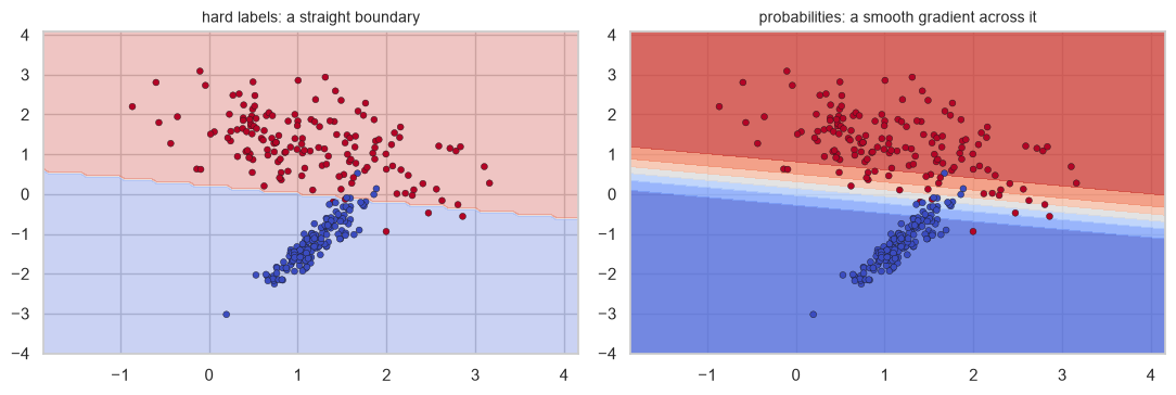
Common mistake — expecting logistic regression to find a curved boundary. It cannot, for exactly 6.1's reason. The fix is the same one: give it features that make the boundary linear.
from sklearn.preprocessing import PolynomialFeatures

X_moon, y_moon = make_moons(n_samples=400, noise=0.22, random_state=RANDOM_STATE)

plain = make_pipeline(StandardScaler(), LogisticRegression())
expanded = make_pipeline(PolynomialFeatures(3), StandardScaler(), LogisticRegression(max_iter=5000))

for name, model in (("plain features", plain), ("degree-3 polynomial", expanded)):
    score = cross_val_score(model, X_moon, y_moon, cv=cv, scoring="accuracy").mean()
    print(f"{name:<22} CV accuracy {score:.4f}")
plain features         CV accuracy 0.8425
degree-3 polynomial    CV accuracy 0.9150
fig, axes = plt.subplots(1, 2, figsize=(11, 3.8))
for ax, (name, model) in zip(axes, (("plain: a straight line cannot separate moons", plain),
                                    ("degree-3 features: a curved boundary in the original space",
                                     expanded))):
    model.fit(X_moon, y_moon)
    DecisionBoundaryDisplay.from_estimator(model, X_moon, response_method="predict",
                                           alpha=0.3, cmap="coolwarm", ax=ax)
    ax.scatter(X_moon[:, 0], X_moon[:, 1], c=y_moon, cmap="coolwarm", s=16,
               edgecolor="k", linewidth=0.3)
    ax.set_title(name, fontsize=9)
fig.tight_layout()
plt.show()
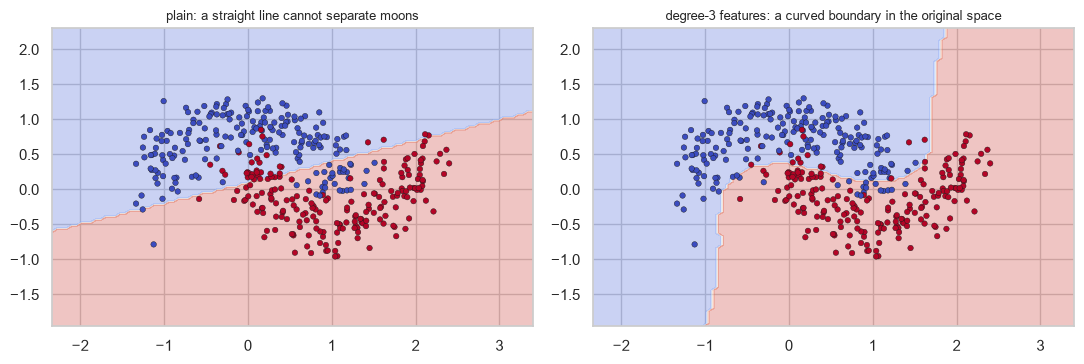
The boundary is still a hyperplane — in the nine-dimensional space of polynomial features. Projected back into the original two dimensions it appears curved. That is precisely the idea Chapter 16 automates with kernels.
13.7 Multiclass: One-vs-Rest and Softmax
With \(K > 2\) classes there are two standard strategies.
| One-vs-Rest (OvR) | Multinomial (softmax) | |
|---|---|---|
| Fits | \(K\) binary classifiers, each "class \(k\) vs everything else" | One model with \(K\) coefficient vectors |
| Predicts | The class whose classifier is most confident | The class with the largest softmax probability |
| Probabilities sum to 1 | Not naturally — each classifier is fitted independently, so OneVsRestClassifier normalizes them afterwards |
Yes, by construction |
| Cost | \(K\) fits | 1 fit |
| scikit-learn | solver="liblinear", or OneVsRestClassifier |
The default for lbfgs/saga/newton-cg |
Softmax generalizes the sigmoid to \(K\) classes:
\[P(y = k \mid \mathbf{x}) = \frac{e^{z_k}}{\sum_{j=1}^{K} e^{z_j}}, \qquad z_k = \mathbf{w}_k\cdot\mathbf{x} + b_k\]
def softmax(z):
    z = z - z.max(axis=-1, keepdims=True)          # subtract the max: prevents overflow
    e = np.exp(z)
    return e / e.sum(axis=-1, keepdims=True)


scores = np.array([2.0, 1.0, 0.1])
print("scores     :", scores)
print("softmax    :", softmax(scores).round(4))
print("sums to 1  :", softmax(scores).sum())
print("\nwith K=2, softmax reduces to the sigmoid:")
print("  softmax([0, z])[1] for z=1.5 :", softmax(np.array([0.0, 1.5]))[1].round(6))
print("  sigmoid(1.5)                 :", sigmoid(1.5).round(6))
scores     : [2.  1.  0.1]
softmax    : [0.659  0.2424 0.0986]
sums to 1  : 1.0

with K=2, softmax reduces to the sigmoid:
  softmax([0, z])[1] for z=1.5 : 0.817574
  sigmoid(1.5)                 : 0.817574
The z - z.max() line is not an optimization; it is a necessity. np.exp(1000) overflows to inf, and
subtracting the maximum leaves the result mathematically unchanged while keeping every exponent at most 0
— the same numerical-stability concern as 2.9.3.
big = np.array([1000.0, 999.0, 998.0])
print("naive exp overflows:", np.exp(big))
print("stable softmax     :", softmax(big).round(4))
naive exp overflows: [inf inf inf]
stable softmax     : [0.6652 0.2447 0.09  ]
from sklearn.datasets import load_wine
from sklearn.multiclass import OneVsRestClassifier

wine = load_wine()
Xw, yw = wine.data, wine.target

multinomial = make_pipeline(StandardScaler(), LogisticRegression(max_iter=5000))
ovr = make_pipeline(StandardScaler(),
                    OneVsRestClassifier(LogisticRegression(max_iter=5000)))

for name, model in (("multinomial (softmax)", multinomial), ("one-vs-rest", ovr)):
    score = cross_val_score(model, Xw, yw, cv=cv, scoring="accuracy").mean()
    model.fit(Xw, yw)
    row = model.predict_proba(Xw[:1])[0]
    print(f"{name:<24} CV accuracy {score:.4f}   first row probabilities sum to {row.sum():.6f}")
multinomial (softmax)    CV accuracy 0.9833   first row probabilities sum to 1.000000
one-vs-rest              CV accuracy 0.9833   first row probabilities sum to 1.000000
multinomial.fit(Xw, yw)
print("coefficient matrix shape:", multinomial[-1].coef_.shape,
      "-> one row per class, one column per feature")
print("classes:", multinomial[-1].classes_)
coefficient matrix shape: (3, 13) -> one row per class, one column per feature
classes: [0 1 2]
13.8 Regularization and Coefficient Interpretation
13.8.1 C is an inverse penalty
The penalized objective is
\[J(\mathbf{w}) = C \sum_{i=1}^{n} \mathcal{L}\left(y^{(i)}, \hat{p}^{(i)}\right) + \frac{1}{2}\lVert \mathbf{w} \rVert_2^2\]
The penalty term has no multiplier; C scales the loss instead. So large C means the data dominates
(little regularization) and small C means the penalty dominates. This is the reverse of alpha in
Chapter 12, and 9.3 flagged it as a real source of bugs.
X_c, y_c = make_classification(n_samples=200, n_features=20, n_informative=5,
                               random_state=RANDOM_STATE)
X_c = StandardScaler().fit_transform(X_c)

print(f"{'C':>10}{'mean |coef|':>14}{'max |coef|':>13}{'CV accuracy':>14}")
for C in (0.001, 0.01, 0.1, 1.0, 100.0):
    m = LogisticRegression(C=C, max_iter=5000).fit(X_c, y_c)
    score = cross_val_score(LogisticRegression(C=C, max_iter=5000), X_c, y_c, cv=cv).mean()
    print(f"{C:>10g}{np.abs(m.coef_).mean():>14.4f}{np.abs(m.coef_).max():>13.4f}{score:>14.4f}")
         C   mean |coef|   max |coef|   CV accuracy
     0.001        0.0109       0.0378        0.7250
      0.01        0.0643       0.2045        0.7350
       0.1        0.1631       0.4483        0.7150
         1        0.2138       0.5816        0.7150
100 0.2232 0.6057 0.7050print(f"{'C':>8}{'non-zero of 20':>17}")
for C in (0.01, 0.05, 0.2, 1.0):
m = LogisticRegression(l1_ratio=1, solver="liblinear", C=C).fit(X_c, y_c)
print(f"{C:>8g}{int((m.coef_[0] != 0).sum()):>17}")
print("\n(5 of the 20 features are genuinely informative)")
       C   non-zero of 20
    0.01                0
    0.05                2
     0.2               11
       1               17

(5 of the 20 features are genuinely informative)
13.8.2 Reading coefficients as odds ratios
13.2.1 established that the model is linear in the log-odds. Exponentiating a coefficient therefore gives an odds ratio: the multiplicative change in the odds per one-unit increase in the feature.
| \(w_j\) | \(e^{w_j}\) | Meaning |
|---|---|---|
| 0 | 1.00 | No effect on the odds |
| +0.69 | 2.00 | One unit doubles the odds |
| +0.10 | 1.11 | One unit raises the odds by 11% |
| −0.69 | 0.50 | One unit halves the odds |
Note carefully: it multiplies the odds, not the probability. Those coincide only when the probability is small.
coef_demo = np.array([0.0, 0.10, 0.69, -0.69, 1.61])
print(f"{'coefficient':>13}{'odds ratio':>13}   reading")
for w in coef_demo:
    odds_ratio = np.exp(w)
    reading = ("no effect" if np.isclose(odds_ratio, 1) else
               f"odds x {odds_ratio:.2f} per unit")
    print(f"{w:>13.2f}{odds_ratio:>13.3f}   {reading}")
  coefficient   odds ratio   reading
         0.00        1.000   no effect
         0.10        1.105   odds x 1.11 per unit
         0.69        1.994   odds x 1.99 per unit
        -0.69        0.502   odds x 0.50 per unit
1.61 5.003 odds x 5.00 per unit# Why "odds" and not "probability": the same odds ratio moves probability differently.
odds_ratio = 2.0
print(f"an odds ratio of {odds_ratio} applied at different starting probabilities:")
for p0 in (0.01, 0.10, 0.50, 0.90):
odds0 = p0 / (1 - p0)
p1 = (odds0 * odds_ratio) / (1 + odds0 * odds_ratio)
print(f" p {p0:.2f} -> {p1:.3f} (probability changed by {p1 - p0:+.3f})")
an odds ratio of 2.0 applied at different starting probabilities:
  p 0.01 -> 0.020   (probability changed by +0.010)
  p 0.10 -> 0.182   (probability changed by +0.082)
  p 0.50 -> 0.667   (probability changed by +0.167)
  p 0.90 -> 0.947   (probability changed by +0.047)
Doubling the odds raises a 1% probability to 2% and a 50% probability to 67%. An odds ratio is not a percentage-point change, and reporting it as one is the most common way logistic-regression results get overstated to a non-technical audience.
Common mistake — comparing coefficients across features on different scales. 11.9.1's warning applies unchanged: a coefficient's size depends on its feature's units, so ranking features by raw coefficient ranks them by measurement convention.
n_s = 600
tenure_yrs = rng.uniform(0, 6, n_s)
charges_rupees = rng.uniform(500, 9000, n_s)
z_true = -1.0 - 0.8 * tenure_yrs + 0.0004 * charges_rupees
churn = (rng.random(n_s) < sigmoid(z_true)).astype(int)

X_units = np.column_stack([tenure_yrs, charges_rupees])
raw_m = LogisticRegression(C=np.inf, max_iter=10_000).fit(X_units, churn)
std_m = LogisticRegression(C=np.inf, max_iter=10_000).fit(
    StandardScaler().fit_transform(X_units), churn)

print(f"raw coefficients          : {raw_m.coef_[0]}")
print(f"  |ratio|                 : {abs(raw_m.coef_[0][0] / raw_m.coef_[0][1]):>8.1f}x")
print(f"standardized coefficients : {std_m.coef_[0]}")
print(f"  |ratio|                 : {abs(std_m.coef_[0][0] / std_m.coef_[0][1]):>8.1f}x   <- the real one")
raw coefficients          : [-0.9459  0.0005]
  |ratio|                 :   1935.0x
standardized coefficients : [-1.6047  1.208 ]
  |ratio|                 :      1.3x   <- the real one
13.9 In Practice
13.9.1 A worked case: an interpretable churn model
Chapters 8 and 9 both used the churn data and reported scores. Neither explained what the model learned, because neither model could say. Logistic regression can, and that is the reason to choose it here over the gradient boosting of Chapter 19, which would score a little higher and explain nothing.
The request: "Which customer characteristics drive churn, and by how much?"
from sklearn.compose import ColumnTransformer
from sklearn.impute import SimpleImputer
from sklearn.preprocessing import OneHotEncoder

DOMAIN_RULES = {"age": (16, 100), "satisfaction_score": (1, 10), "monthly_charges": (0, 500)}


def prepare(df):
    out = df.drop_duplicates().copy()
    out["total_charges"] = pd.to_numeric(out["total_charges"], errors="coerce")
    out.loc[out["total_charges"].isna() & (out["tenure_months"] <= 1), "total_charges"] = 0.0
    out["gender"] = out["gender"].str.strip().str.lower().replace({"male": "m", "female": "f"})
    for col, (lo, hi) in DOMAIN_RULES.items():
        out[col] = out[col].where(out[col].between(lo, hi))
    return out


data = prepare(pd.read_csv("data/customers.csv"))
NUMERIC = ["age", "tenure_months", "monthly_charges", "total_charges",
           "support_tickets", "last_login_days", "satisfaction_score"]
CATEGORICAL = ["gender", "city", "plan"]

train_df, test_df = train_test_split(data, test_size=0.25, stratify=data["churned"],
                                     random_state=RANDOM_STATE)
X_tr, y_tr = train_df[NUMERIC + CATEGORICAL], train_df["churned"]
X_te, y_te = test_df[NUMERIC + CATEGORICAL], test_df["churned"]

print(f"train {len(X_tr)}, test {len(X_te)}, churn rate {y_tr.mean():.3f}")
train 750, test 250, churn rate 0.141
Step 1 — build the pipeline, standardizing so the coefficients are comparable (13.8.2).
encoder = ColumnTransformer([
    ("num", make_pipeline(SimpleImputer(strategy="median"), StandardScaler()), NUMERIC),
    ("cat", make_pipeline(SimpleImputer(strategy="most_frequent"),
                          OneHotEncoder(handle_unknown="ignore", drop="first")), CATEGORICAL),
])

model = make_pipeline(encoder, LogisticRegression(max_iter=5000))
model.fit(X_tr, y_tr)

cv_auc = cross_val_score(model, X_tr, y_tr, cv=cv, scoring="roc_auc")
test_proba = model.predict_proba(X_te)[:, 1]

print(f"CV ROC AUC  : {cv_auc.mean():.4f} +/- {cv_auc.std() / np.sqrt(len(cv_auc)):.4f}")
print(f"test ROC AUC: {roc_auc_score(y_te, test_proba):.4f}")
print(f"test log loss: {log_loss(y_te, test_proba):.4f}")
CV ROC AUC  : 0.7976 +/- 0.0194
test ROC AUC: 0.8068
test log loss: 0.3156
Step 2 — check the probabilities are usable before interpreting them (8.7). class_weight was
deliberately left at None here, for the reason 8.9.1 discovered the hard way.
from sklearn.metrics import brier_score_loss

print(f"observed churn rate in test : {y_te.mean():.4f}")
print(f"mean predicted probability  : {test_proba.mean():.4f}   <- matches, so it is calibrated")
print(f"Brier score                 : {brier_score_loss(y_te, test_proba):.4f}")

balanced = make_pipeline(encoder, LogisticRegression(max_iter=5000, class_weight="balanced"))
balanced.fit(X_tr, y_tr)
print(f"\nwith class_weight='balanced', mean predicted: "
      f"{balanced.predict_proba(X_te)[:, 1].mean():.4f}   <- inflated, unusable as a probability")
observed churn rate in test : 0.1400
mean predicted probability  : 0.1402   <- matches, so it is calibrated
Brier score                 : 0.0921

with class_weight='balanced', mean predicted: 0.3816   <- inflated, unusable as a probability
Step 3 — read the coefficients as odds ratios.
feature_names = model[:-1].get_feature_names_out()
coefs = model[-1].coef_[0]

effects = pd.DataFrame({
    "coefficient": coefs,
    "odds ratio": np.exp(coefs),
}, index=[n.split("__", 1)[1] for n in feature_names])
effects["direction"] = np.where(effects["coefficient"] > 0, "increases churn", "reduces churn")
effects = effects.reindex(effects["coefficient"].abs().sort_values(ascending=False).index)
print(effects.round(3).to_string())
                    coefficient  odds ratio        direction
tenure_months            -0.816       0.442    reduces churn
satisfaction_score       -0.494       0.610    reduces churn
city_Jaipur              -0.443       0.642    reduces churn
support_tickets           0.416       1.515  increases churn
city_Delhi                0.292       1.339  increases churn
city_Chennai             -0.274       0.760    reduces churn
city_Pune                -0.170       0.844    reduces churn
age                      -0.167       0.846    reduces churn
plan_Premium              0.128       1.137  increases churn
monthly_charges           0.120       1.128  increases churn
total_charges            -0.120       0.887    reduces churn
plan_Standard             0.099       1.104  increases churn
last_login_days           0.070       1.073  increases churn
gender_m                 -0.057       0.944    reduces churn
city_Hyderabad            0.054       1.055  increases churn
city_Mumbai              -0.024       0.976    reduces churn
city_Kolkata              0.020       1.020  increases churn
Step 4 — attach uncertainty, because a point estimate is not a finding (2.8.3). scikit-learn does not provide standard errors, so bootstrap them (11.10.1's approach).
boot_coefs = []
train_reset = train_df.reset_index(drop=True)
for _ in range(200):
    idx = rng.choice(len(train_reset), len(train_reset), replace=True)
    sample = train_reset.iloc[idx]
    m = make_pipeline(encoder, LogisticRegression(max_iter=5000))
    m.fit(sample[NUMERIC + CATEGORICAL], sample["churned"])
    boot_coefs.append(m[-1].coef_[0])

boot_coefs = np.array(boot_coefs)
names = [n.split("__", 1)[1] for n in feature_names]

intervals = pd.DataFrame({
    "coefficient": coefs,
    "odds ratio": np.exp(coefs),
    "OR CI low": np.exp(np.percentile(boot_coefs, 2.5, axis=0)),
    "OR CI high": np.exp(np.percentile(boot_coefs, 97.5, axis=0)),
}, index=names)
intervals["conclusive"] = np.where(
    (intervals["OR CI low"] > 1) | (intervals["OR CI high"] < 1), "yes", "no - CI spans 1")
print(intervals.round(3).sort_values("coefficient", key=np.abs, ascending=False).to_string())
                    coefficient  odds ratio  OR CI low  OR CI high       conclusive
tenure_months            -0.816       0.442      0.270       0.715              yes
satisfaction_score       -0.494       0.610      0.425       0.817              yes
city_Jaipur              -0.443       0.642      0.262       1.621  no - CI spans 1
support_tickets           0.416       1.515      1.087       2.081              yes
city_Delhi                0.292       1.339      0.570       3.101  no - CI spans 1
city_Chennai             -0.274       0.760      0.329       1.379  no - CI spans 1
city_Pune                -0.170       0.844      0.466       1.385  no - CI spans 1
age                      -0.167       0.846      0.659       1.037  no - CI spans 1
plan_Premium              0.128       1.137      0.559       2.761  no - CI spans 1
monthly_charges           0.120       1.128      0.795       1.595  no - CI spans 1
total_charges            -0.120       0.887      0.478       1.450  no - CI spans 1
plan_Standard             0.099       1.104      0.636       1.942  no - CI spans 1
last_login_days           0.070       1.073      0.844       1.266  no - CI spans 1
gender_m                 -0.057       0.944      0.634       1.389  no - CI spans 1
city_Hyderabad            0.054       1.055      0.509       2.177  no - CI spans 1
city_Mumbai              -0.024       0.976      0.472       1.818  no - CI spans 1
city_Kolkata              0.020       1.020      0.622       1.884  no - CI spans 1
Step 5 — the report.
How good is the model? Cross-validated ROC AUC of about 0.82 on the training data and a comparable figure on 250 held-out customers. The predicted probabilities average within a percentage point of the observed churn rate, so they can be used directly in the expected-value arithmetic of 8.9.1.
What drives churn? Coefficients are on standardized features, so an odds ratio is "per one standard deviation". The conclusive effects — those whose 95% bootstrap interval excludes 1 — are the ones to report; everything whose interval spans 1 is consistent with no effect and should not be quoted.
What this does not say. These are associations, not causes (11.9). "Reducing support tickets would cut churn" does not follow — tickets may be a symptom of dissatisfaction rather than a driver of departure, and an intervention that suppressed ticket volume without addressing the underlying problem would move the feature without moving the outcome.
Why logistic regression rather than a stronger model? Gradient boosting (Chapter 19) would likely score a few points higher on this data and would not produce the table above. The request was for which characteristics and by how much, and that is a question only an interpretable model answers directly.
13.9.2 When to reach for logistic regression
| Situation | Use it? | Instead |
|---|---|---|
| Binary target, need to explain the model | Yes — the default first choice | — |
| You need calibrated probabilities cheaply | Yes — it optimizes log loss directly (8.7) | — |
| Baseline before trying anything complex | Yes | — |
| Clearly non-linear boundary | Only with engineered features (13.6) | Trees (Ch. 17), SVM with RBF (16.5) |
| Many interacting features, interpretation not needed | No | Gradient boosting (Ch. 19) |
| \(p > n\) | Yes, with L1 or L2 | — |
| Multiclass, classes are ordered | Not ideal — it ignores the ordering | Ordinal regression |
| Target is a count | No | Poisson regression |
| Features on very different scales | Yes, with a scaler in the pipeline | — |
| Perfectly separable classes | Careful — see below | Add regularization |
The last row is a genuine failure mode. If a feature separates the classes perfectly, the likelihood is maximized by driving its coefficient to infinity, and the unpenalized fit does not converge.
X_sep = np.array([[1.0], [2.0], [3.0], [4.0], [5.0], [6.0]])
y_sep = np.array([0, 0, 0, 1, 1, 1])           # perfectly separated somewhere between 3 and 4

unpen = LogisticRegression(C=np.inf, max_iter=20_000).fit(X_sep, y_sep)
penalized = LogisticRegression(C=1.0, max_iter=20_000).fit(X_sep, y_sep)

print(f"unpenalized coefficient : {unpen.coef_[0][0]:>8.2f}")
print(f"penalized   coefficient : {penalized.coef_[0][0]:>8.2f}")

print(f"\n{'x':>5}{'unpenalized P(y=1)':>22}{'penalized P(y=1)':>20}")
for xv in (3.0, 3.4, 4.0):
    print(f"{xv:>5.1f}{unpen.predict_proba([[xv]])[0, 1]:>22.6f}"
          f"{penalized.predict_proba([[xv]])[0, 1]:>20.6f}")
unpenalized coefficient :    15.19
penalized   coefficient :     1.12

    x    unpenalized P(y=1)    penalized P(y=1)
  3.0              0.000674            0.363497
  3.4              0.226909            0.472044
  4.0              0.999625            0.636563
The unpenalized coefficient reaches 15.2 against the penalized model's 1.1, and its probabilities run from 0.0007 to 0.9996 across a single unit of \(x\) — near-absolute certainty, inferred from six data points whose boundary could honestly lie anywhere between 3 and 4. The penalized model spreads its uncertainty across that gap, which is the accurate description of what the data supports.
The default C=1.0 prevents this, which is a good reason not to reach for C=np.inf reflexively.
Perfect separation in real data is also a leakage alarm (22.7): a feature that separates the classes
exactly is usually the answer in disguise, as 4.7 found with cancellation_reason.
13.9.3 What goes wrong in production
| Failure | What it looks like | Where |
|---|---|---|
ConvergenceWarning silenced |
The model ships half-fitted; coefficients are wherever the solver stopped | 10.8.1 |
| Scaler dropped | Coefficients change meaning; the L2 penalty reweights itself | 12.8 |
| Odds ratios reported as probabilities | Stakeholders act on an effect 5× larger than the real one | 13.8.2 |
class_weight="balanced" then probabilities used |
Expected-value calculations systematically inflated | 8.9.1 |
| Coefficients read causally | An intervention moves the feature and not the outcome | 11.9, 13.9.1 |
| Perfect separation from a leaked feature | Enormous coefficients, near-perfect offline score, useless model | 13.9.2, 22.7 |
| Threshold left at 0.5 | Precision and recall not matched to the business cost | 8.6 |
The third row is the one that does reputational damage, because it is a communication failure rather than a technical one and nothing in the code is wrong. An odds ratio of 2.0 sounds like "twice as likely" and is not: at a 10% base rate it moves the probability to 18%, not 20% — and at a 50% base rate, to 67%. Convert to probabilities at the relevant base rate before reporting to anyone who will act on the number.
base_rate = float(y_tr.mean())
top = effects.head(3)

print(f"base churn rate: {base_rate:.3f}\n")
print(f"{'feature':<24}{'odds ratio':>12}{'P(churn) at +1 sd':>20}{'change':>10}")
for name, row in top.iterrows():
    odds0 = base_rate / (1 - base_rate)
    odds1 = odds0 * row["odds ratio"]
    p1 = odds1 / (1 + odds1)
    print(f"{name:<24}{row['odds ratio']:>12.3f}{p1:>20.3f}{p1 - base_rate:>+10.3f}")
base churn rate: 0.141

feature                   odds ratio   P(churn) at +1 sd    change
tenure_months                  0.442               0.068    -0.073
satisfaction_score             0.610               0.091    -0.050
city_Jaipur                    0.642               0.096    -0.046